STWAVE Model

Florida Public Flood Loss Model

FPFLM

Primary Document

Contents

1 General Description of the STWAVE Model
2 Technical Description of the STWAVE Model
3 Computer Model Design & Implementation
4 References

General Description of the STWAVE Model

STWAVE (STeady State spectral WAVE model) is a purely steady-state model, which is appropriate for relatively short distances or times. Changing winds and water levels can be included by computing a series of steady-state conditions. For hurricanes, STWAVE requires offshore wave heights from another model, which are taken as the boundary conditions. STWAVE will then compute wave heights through to the shoreline, or overland if a region is flooded. STWAVE has also been widely used for FEMA Flood Insurance Rate Map (FIRM) studies.

Wave computations for this project used a slightly modified version of the STWAVE spectral wave model (Smith et al., 2001). Modifications included spectral irregular wave breaking using the Thornton and Guza (1983) formulation, and wave dissipation by vegetation using the Mendez and Losada (2004) representation. Bottom friction used a Manning-type formulation with values dependent on land use/land cover type. For all grid locations, values needed to be determined for elevation, and land use/land cover. The land use values were used to create values for Manning’s coefficient, at all grid locations, in addition to estimates for vegetation stem density, diameter, and height.

Technical Description of the STWAVE Model

Bottom Friction

Bottom frictional dissipation arises from the rough boundary (rocks, sand, vegetation) that waves encounter as they propagate across the seabed and overland. It is usually represented in wave models using a spatially-varying friction coefficient or Manning’s n parameter that is dependent on vegetation or sea bed type, or land use activities. These are often extracted from USGS GAP databases (http://gapanalysis.usgs.gov/data/), but will require significant effort to create representative grids. STWAVE features spatially-varying bottom friction that may be used without modification. For the purposes of the FPHLM, computational wave grids were created including Manning’s n parameters that vary depending on the land use/land cover databases.

Wave Dissipation by Vegetative-Like Objects

Almost all wave models were designed to be used in open sea areas where there are no houses, trees, fences, or other objects found in flooded land areas. For these reasons, they have been found to underestimate wave dissipation in overland regions, particularly over long distances (Tomiczek et al., 2014). For these reasons, we have incorporated additional sources of dissipation into the wave model. These mechanisms include dissipation against the stems of bushes and trunks and branches of trees; by houses and other buildings; and by other aspects of the built environment such as utility poles, fences, and so on.

Of these, dissipation by vegetation is the most direct to implement. Using a Morison-equation type formulation, this can be added into the wave model as an additional dissipative source with moderate coding. The details would likely follow Mendez and Losada (2004) as volumetric dissipation over the water depth, with appropriate geometrical considerations applied from knowledge of the obstacles. The most difficult aspect of this will be determining the appropriate coefficients for various vegetation types, and determining from land cover/land use or other data how to assign these coefficients for a specific location. This will require significant effort as part of the grid generation process.

The final source of overland dissipation is from other aspects of the built environment, which include utility poles, fences, cars, landscaping features, and so on. It should be emphasized that no existing models consider this type of dissipation and we will be exploring very new territory. Details of objects leading to dissipation will likely be very difficult to determine with great accuracy for a given location, and it may be necessary to create representative cases for different land use types. Actual dissipation will likely follow Morison-equation type formulations and may be treated as variations on Mendez and Losada (2004) type dissipation.

Dissipation in the Mendez formulation is dependent on a variety of parameters: (1) the drag coefficient, Cd (dimensionless); (2) the frontal area per unit height of the dissipation, bv (meters), which is like a diameter; (3) the number of dissipators per unit ground area, N (1/meter²), and the vegetation height, αh (meters). With the exception of drag coefficients, which have a relatively small range of variation, these are all measurable physical quantities, and may be evaluated for various land use/land cover types. It is, however, expected that there will be a significant range of variation between specific sites with similar land use or land cover, and we will attempt to categorize the likely range of variation. Table 1 gives parameter values used here for Manning’s n and vegetative dissipation relating to land use/land cover types.

Table 1. National Land Cover Database Descriptions and Values used

Description	ID	Manning’s n	CdbvN (m^-1)	Vegetation Height (m)
Open Water	11	0.025	0	0
Developed Open Space	20	0.035	0.02	1
Developed Low Intensity	22	0.120	0.075	10
Developed Medium Intensity	23	0.120	0.1	10
Developed High Intensity	24	0.120	0.15	10
Barren Land	31	0.030	0.01	0.05
Deciduous Forest	41	0.160	0.05	15
Evergreen Forest	42	0.180	0.05	15
Mixed Forest	43	0.170	0.05	15
Shrub/Scrub	52	0.080	0.1	2
Grassland/Herbaceous	71	0.035	0.03	0.1
Pasture/Hay	81	0.050	0.3	0.5
Cultivated Crops	82	0.100	0.3	0.4
Woody Wetlands	90	0.150	0.3	3
Emergent Herbaceous Wetlands	91	0.055	0.1	0.4

Wave Breaking

Spectral wave breaking dissipation is needed for the FPHLM to ensure that wave heights decrease in shallow depths and while propagating overland. Because the standard version of STWAVE uses a very simple depth-limited breaking method that simply imposes whenever wave heights become too large relative to depth.

STWAVE requires modifications (which have already been implemented by FPHLM workers) to its breaking mechanisms to give good results for the FPHLM. These modifications use well-known and accepted breaking representations: the final breaking formulation chosen is the bulk dissipation representation of Thornton and Guza (1983). For the purposes of the FPHLM, breaking will be most important at the shoreline when wave height/depth ratios are large, and least important in regions where the wave height is small.

Bottom Friction

Bottom frictional dissipation arises from the rough boundary (rocks, sand, vegetation) that waves encounter as they propagate across the seabed and overland. It is usually represented in wave models using a spatially-varying friction coefficient or Manning’s n parameter that is dependent on vegetation or sea bed type, or land use activities. These are often extracted from USGS GAP databases (http://gapanalysis.usgs.gov/data/), but will require significant effort to create representative grids. STWAVE features spatially-varying bottom friction that may be used without modification. For the purposes of the FPHLM, computational wave grids will be created that include Manning’s n parameters that vary depending on the land use/land cover databases.

Wave Dissipation by Vegetative-Like Objects

Almost all wave models were designed to be used in open sea areas where there are no houses, trees, fences, or other objects found in flooded land areas. For these reasons, they have been found to underestimate wave dissipation in overland regions, particularly over long distances (Tomiczek et al., 2014). For these reasons, we will investigate additional dissipative mechanisms in flooded regions, and how to incorporate these into wave models. These mechanisms include dissipation against the stems of bushes and trunks and branches of trees; by houses and other buildings; and by other aspects of the built environment such as utility poles, fences, and so on.

Of these, dissipation by vegetation is the most direct to implement. Using a Morison-equation type formulation, this can be added into the wave model as an additional dissipative source with moderate coding. The details would likely follow Mendez et al. (2004) as volumetric dissipation over the water depth, with appropriate geometrical considerations applied from knowledge of the obstacles. The most difficult aspect of this will be determining the appropriate coefficients for various vegetation types, and determining from land cover/land use or other data how to assign these coefficients for a specific location. This will require significant effort as part of the grid generation process.

Dissipation in the Mendez et al. formulation is dependent on a variety of parameters: (1) the drag coefficient, Cd (dimensionless); (2) the frontal area per unit height of the dissipation, bv (meters), which is like a diameter; (3) the number of dissipators per unit ground area, N (1/meter²), and the vegetation height, αh (meters). With the exception of drag coefficients, which have a relatively small range of variation, these are all measurable physical quantities, and may be evaluated for various land use/land cover types. It is, however, expected that there will be a significant range of variation between specific sites with similar land use or land cover, and we will attempt to categorize the likely range of variation.

Computational Examples – Wave Dissipation Over a Flat Bed

The effects of various dissipation mechanisms can be demonstrated using the simple example of wave dissipation over a flat bed with no wind input. All waves have an initial significant wave height of H_s=1m, peak period of T_p=10s, and propagate over a flat bed with depth 2m. Five cases with different dissipation were examined:

Case	Description	Breaking Type	Manning’s n	C_db_vN (m^-1)	Veg. Height (m)
1	Original	Depth-Limited	0	0	0
2	Breaking only	Thornton/Guza	0	0	0
3	Scattered Vegetation	Thornton/Guza	0.02	0.01	1
4	Medium Vegetation	Thornton/Guza	0.05	0.1	1
5	Dense Vegetation	Thornton/Guza	0.015	0.3	2

Figure 1 shows computed wave heights using the modified STWAVE model for cases 1-5. The unmodified model of Case 1 has waves that are too small to be dissipated under the simple depth-limited breaking criterion, and propagates essentially unchanged over the flat bed. This is not at all realistic for waves overland, and demonstrates why changes were necessary. Case 2, with Thornton and Guza breaking only, shows strong dissipation at the shoreline where wave height/depth ratios are large, but then much less dissipation further inland. By 500m inland, wave heights are almost 50 percent lower than with the original formulation. Case 3 adds scattered vegetation to the simulation for both bottom friction and Mendez and Losada form drag dissipation. This gives wave heights only marginally smaller than breaking only computations, and suggests that for low friction/vegetation cases, there is little effect. However, Case 4, which simulates medium vegetation, predicts significant additional dissipation: by 500m inland, wave height have decayed by almost 70 percent. The dense vegetation of Case 5 shows extremely large dissipation, with wave heights decaying by almost 90 percent when compared to shoreline values. Overall, this example shows that vegetative effects are extremely important as distance from the shoreline increases, and in medium and dense vegetative regimes. Near to the shoreline, wave breaking dominates, but even here large differences can be seen less than 100m from the beginning of the simulation. For flooded regions, it appears that these dissipative effects are necessary to achieve increased accuracy.

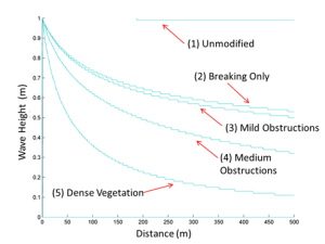
Figure 1. Example of wave dissipation over a flat bed

Application to Florida Coast

For the present model, the coastline of Florida is divided into 116 overlapping subgrids with 20m resolution, each of which can be run separately. It is necessary to divide the coast into subgrids both because not all areas have high surge and waves that need STWAVE computations, but also because STWAVE uses a rectangular grid that does not work well over domains the size of Florida. Figure 2 shows the subgrids, which are both on the open coast, and on inland bays that may see some wave action. With so many storms and subgrids, there are potentially millions of possible STWAVE runs, so some ways must be found to make computations feasible. This is done by:

1. Not computing wave heights in any subgrid where all surge elevations in that grid are less than 0.75m. This is justifiable based on observations that surge of less than 0.75m maximum almost never causes damage in historical storms.

2. Initializing the wave heights and periods at the offshore boundaries of the subdomains based on peak wind velocities at the boundaries, representative water depths, and representative wave fetch lengths (Young and Verhagen, 1996). This is justifiable because the wave heights at insured properties are almost entirely dependent on dissipation by wave breaking and other dissipation, and are almost completely insensitive to initial wave heights once overland. Figure 3 shows an example for different initial offshore wave heights, demonstrating the negligible dependency of initial wave heights in shallow water..

3. Computing full directional spreading, but only at the peak frequency. This is justifiable to include wave refraction and directional spreading around obstacles, but reduces costs compared to a full frequency-directional spectrum.

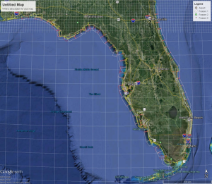
Figure 2. 116 STWAVE subgrids around the coast of Florida

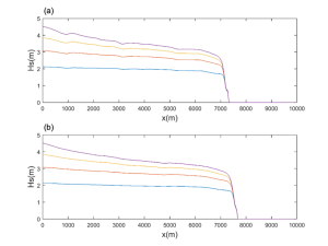
Figure 3. Wave heights along two test transects, with different offshore wave heights. Wave heights in shallow water (~7100m on top subfigure, ~7400m on bottom subfigure) show almost no dependence on initial wave heights.

STWAVE runs are initialized using surge output water levels from the CEST model as provided, and with maximum wind speeds at the offshore boundary. If more than one CEST grid covers a subgrid, the maximum of the two surges is used as initial water level. Once all runs are completed, the results are consolidated for interpolation to exposure locations.

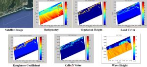
Figure 4. Example of a single wave run on subgrid 1, showing intermediate products and resulting wave heights

Computer Model Design & Implementation

Use Case View of the STWAVE Model

A. Actors:

The use case of the STWAVE model has only one actor: Scientist.

B. Use Case:

The STWAVE model is aimed at calculating the wave height for different regions if flooded by using different grid types and combination types (max. surge and max. wind, and max. wind and surge at max. wind). The model uses surge, wind, location (latitude and longitude), friction, depth and vegetation data.

C. Use Case Diagram:

Figure 2: Use case diagram for STWAVE Model

STWAVE Model Implementation

This model is implemented using MATLAB and FORTRAN programming languages. This section includes the overall flow chart of STWAVE model’s implementation.

Program Flowchart for STWAVE Model

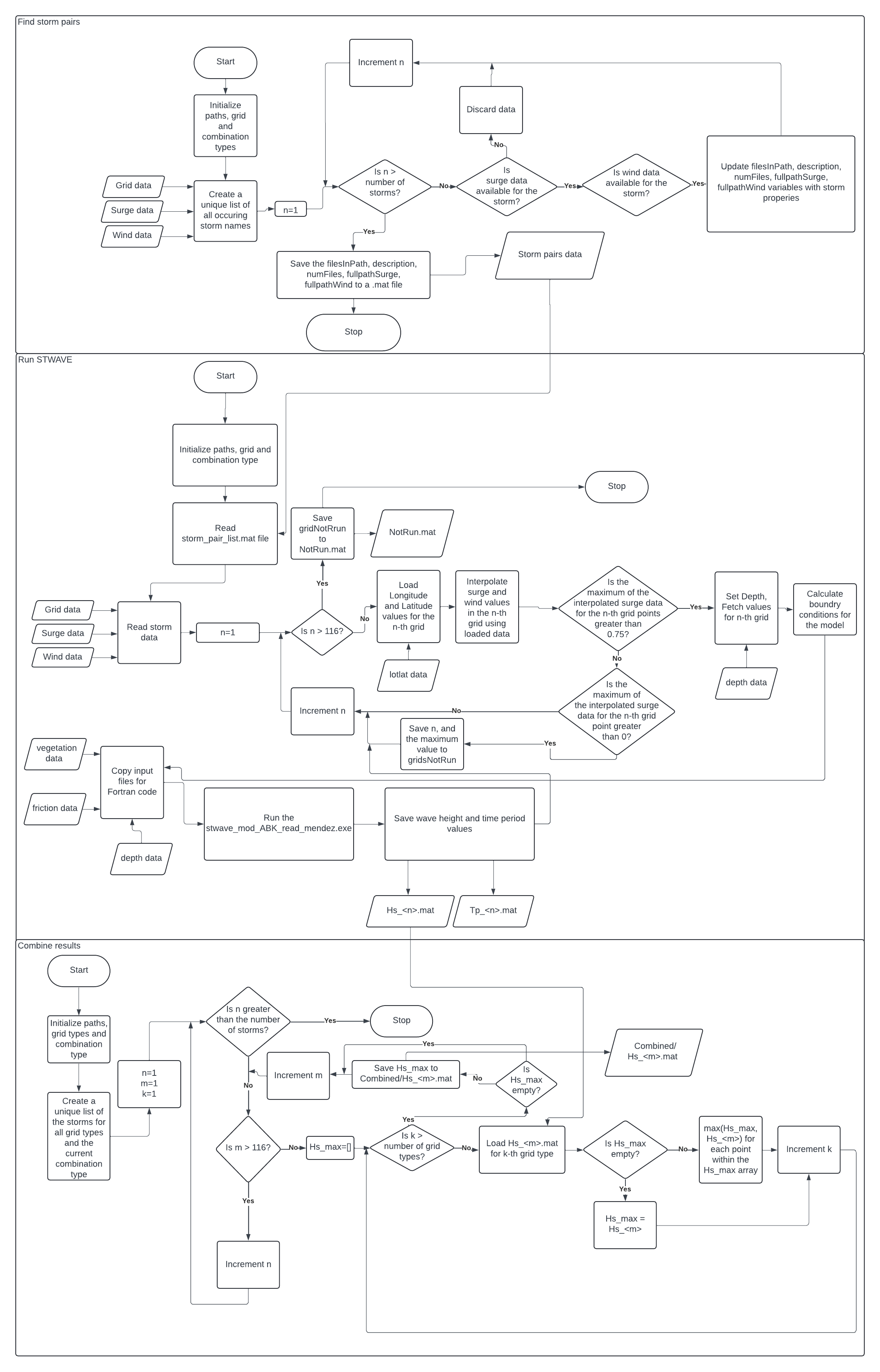
Figure 3: Flowchart for STWAVE Model

Class Diagram and Description

A. Class Diagram

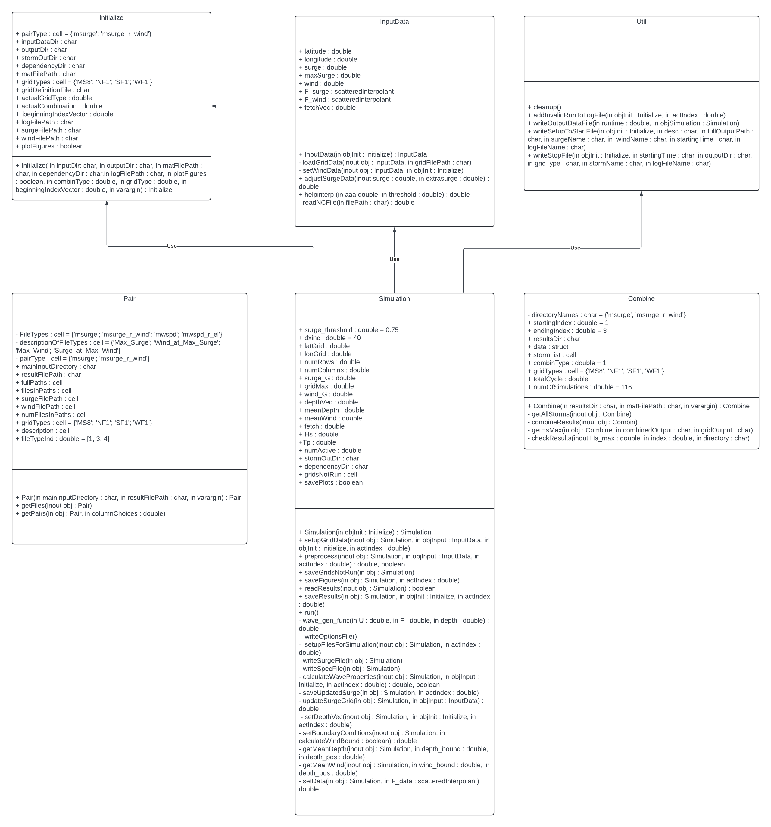
Figure 4: Class diagram for STWAVE Model

B. Class Description

Pair: In order to run the STWAVE model, there needs to be one surge input and one wind input for the same storm. Therefore a check needs to be made to identify the necessary files. are available. This program will cross reference the directories to find the matching input files.The necessary information of the storm, surge and wind data will be saved in a .mat file.
Simulation: Generates and copies the necessary input files to the right location for the STWAVE FORTRAN program, runs the model, and parses and saves the FORTRAN code output to Hs_<index>.mat files.
Initialize: Manages the paths of the necessary input data, and sets the grid and combination types and flags for the model.
InputData: Loads and handles the input data for the STWAVE model.
Util: Handles utility operations, contains static functions only.
Combine: Combines the results for each storm and region. It checks all grid types (AP8, EJX7, HMI41, TP3), and takes the maximum wave height for each point in a region. The surge and max. wind, and max. wind and surge at max. wind combinations are combined separately.

Data Flow Diagram

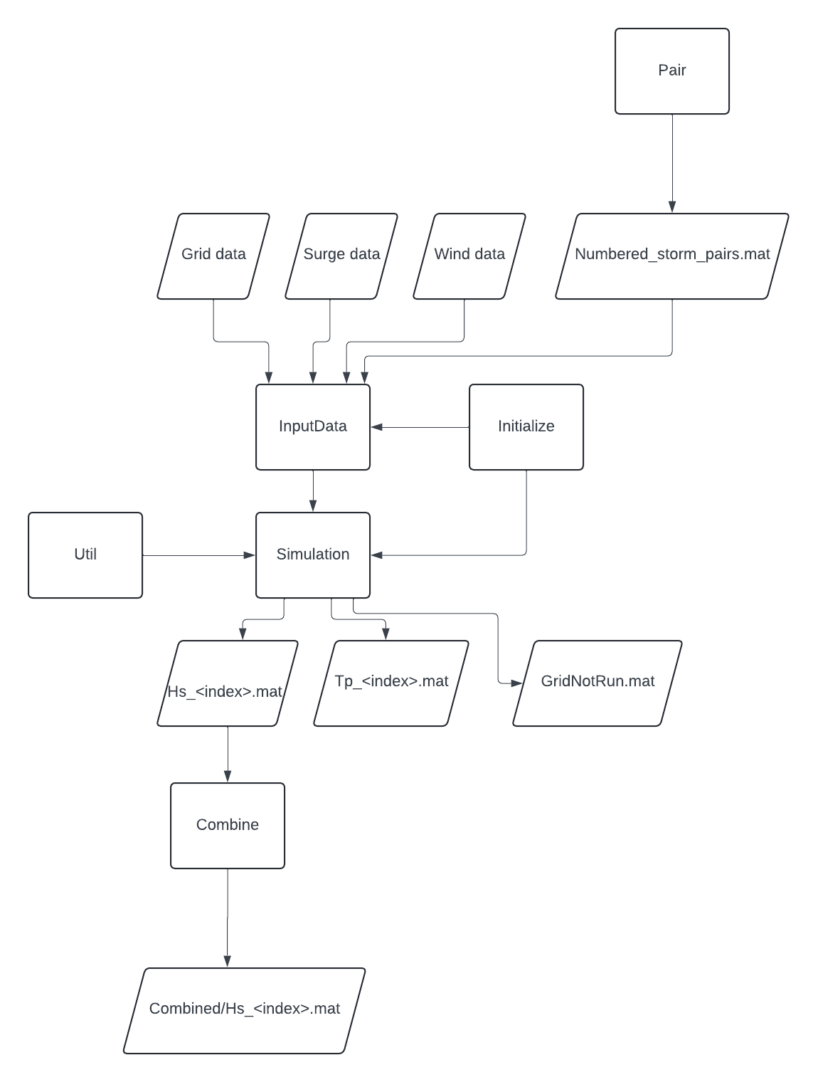
Figure 5: Data Flow Diagram for STWAVE Model

STWAVE Model output

The output files are Hs_<n>.mat files, and n means the n-th region (grid points) where the wave height is calculated if flooded. The content of the MATLAB binary .mat file is an array containing the wave height for each grid point for the n-th location. For example:

1.4700000 1.4700000 1.4700000 1.4700000 1.4700000 1.4700000 1.4700000 1.4700000 …

1.4600000 1.4600000 1.4600000 1.4600000 1.4600000 1.4600000 1.4600000 1.4700000 …

1.4600000 1.4600000 1.4600000 1.4600000 1.4600000 1.4600000 1.4600000 1.4600000 …

1.4500000 1.4500000 1.4500000 1.4600000 1.4600000 1.4600000 1.4600000 1.4600000 …

1.4500000 1.4500000 1.4500000 1.4500000 1.4600000 1.4600000 1.4600000 1.4600000 …

1.4500000 1.4500000 1.4500000 1.4500000 1.4500000 1.4500000 1.4500000 1.4500000 …

1.4400001 1.4400001 1.4500000 1.4500000 1.4500000 1.4500000 1.4500000 1.4400001 …

1.4400001 1.4400001 1.4400001 1.4400001 1.4500000 1.4500000 1.4400001 1.4400001 …

1.4400001 1.4400001 1.4400001 1.4400001 1.4400001 1.4400001 1.4400001 1.4400001 …

1.4400001 1.4400001 1.4400001 1.4400001 1.4400001 1.4400001 1.4400001 1.4299999 …

1.4400001 1.4400001 1.4400001 1.4400001 1.4400001 1.4299999 1.4299999 1.4299999 …

1.4299999 1.4299999 1.4299999 1.4400001 1.4400001 1.4299999 1.4299999 1.4299999 …

1.4299999 1.4299999 1.4299999 1.4299999 1.4299999 1.4299999 1.4299999 1.4299999 …

1.4299999 1.4299999 1.4299999 1.4299999 1.4200000 1.4200000 1.4200000 1.4200000 …

1.4200000 1.4200000 1.4200000 1.4200000 1.4200000 1.4200000 1.4200000 1.4200000 …

…

References

Hope, M., Westerink, J.J., Kennedy, A.B., Kerr, P., Dietrich, J.C., Dawson, C., Bender, C.J., Smith, J., Jensen, R., Zijlema, M., Holthuijsen, L., Luettich, R., Powell, M., Cardone, V., Cox, A.T., Pourtaheri, H., Roberts, H., Atkinson, J., Tanaka, S., Westerink, J., and Westerink, L. (2013). “Hindcast and Validation of Hurricane Ike (2008) Waves, Forerunner, and Storm Surge”, J. Geophys. Res.-Oceans, 118, 4424-4460, doi:10.1002/jgrc.20314.
Mendez, F.J., and Losada, I.J. (2004). “An empirical model to estimate the propagation of random breaking and nonbreaking waves over vegetation fields”. Coastal Engineering, 51(2), 103-118.
Smith, J.M., Sherlock, A.R., and Resio, D.T. (2001). STWAVE: Steady-state spectral wave model user’s manual for STWAVE, Version 3.0. Rept. ERDC/CHL SR-01-1, US Army Corps of Engineers, Engineer Research and Development Center, 81 pp.
Tomiczek, T., Kennedy, A.B., and Rogers, S.P. (2014). “Collapse limit state fragilities of wood-framed residences from storm surge and waves during Hurricane Ike”, J. Waterway, Port, Coastal and Ocean Eng.-ASCE, 140(1), 43-55, doi: 10.1061/(ASCE)WW.1943-5460.0000212.
Young, I.R., and Verhagen, L.A. (1996). “The growth of fetch limited waves in water of finite depth. Part 1. Total energy and peak frequency”. Coastal Eng., 29,. 47-78.