Part IV. Storm Surge Interpolation
Florida Public Flood Loss Model
FPFLM
User Manual
Part VI. Storm Surge Interpolation
Contents
Introduction
The following section includes detailed information about the storm surge interpolation program developed by the storm surge team. The following is a list of the information included in this document:
- Description of the program
- Description of the running environment
- Description of input parameters and files
- Required software and dependencies
- Instructions to run the program
- Description of the outputs of the program
The storm surge interpolation program has two variants, the original implementation and a modified one that allows the code to be run in a distributed fashion on top of Apache Spark. Each one of the implementations has its own characteristics and they will be detailed throughout the document.
Guide Through Storm Surge Interpolation Code
Brief description of the program
The program performs a Barycentric interpolation algorithm for all the points of interest (expressed as latitude and longitude coordinates), and calculates surge results for each stochastic storm generated by the CEST (Coastal and Estuarine Storm Tide) model.
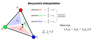
Fig. 1. Graphic representation of the Barycentric interpolation
A typical Barycentric interpolation requires four steps:
- Perform a Delaunay triangulation for the original irregular coordinates. It basically creates a planar object with triangles formed by a given set of points P. E.g.: x1, x2, x3 in Fig. 1;
- For each point of interest p, find in which simplex (triangles formed in 1) does it lie;
- Compute the barycentric coordinates of each point of interest with respect to the vertices of the enclosing simplex (e.g.: λ1, λ2, λ3 in Fig. 1);
- Compute the interpolated value for each point of interest through the barycentric coordinates of the enclosing simplex.
The first three steps are identical for any value we wish to obtain for any set of points of interest. The output of these steps is information about the indices of the vertices and the weights assigned to each point of interest. The fourth step involves the actual interpolation through the weights assigned for each point of interest.
The program is divided into two major stages: mapping and interpolation. The mapping process covers steps 1 through 3, and the interpolation process involves step 4.
Original implementation
The original interpolation program is comprised of four scripts written in Matlab. The scripts can be described as follows:
readENV_interp_only2_nf1_v3.m: this program’s function is to perform the interpolation on locations falls into the NF1 basin
readENV_interp_only2_sf1_v3.m: this program’s function is to perform the interpolation on locations falls into the SF1 basin
readENV_interp_only2_wf1_v3.m: this program’s function is to perform the interpolation on locations falls into the WF1 basin
Required software and dependencies
The original interpolation program requires the following software and packages in order to be able to run:
MATLAB
Add the following lines (matlab path) MatLAB into your ~/.bashrc
export MATLABROOT=/depot/matlab-R2016b/bin
export PATH=$PATH:/depot/matlab-R2016b/bi
Instructions to run the program
The code and previous running environments are located at /home/wilma/Research/Tianyi/FPHLM/surge/. To proceed further, please create your own directory structure using the current env as a reference. You only need to copy over the essential files.
- The assign_basin_zone.ipynb separates the modeler-defined exposure set into three basins (sf1, nf1 and wf1) based on the county_basin_lookup2.csv file.
- In assign_basin_zone.ipynb, several sections generate the interpolation input from different exposure sets, including the modeler-defined exposure set, the notional sets and the validation sets.
- Other directories contain the separated interpolation inputs for previous runs.
- interpolation/code includes the code and running envs of the interpolation program.
- /input has the input for the interpolation program
- /log contains the log of the MATLAB program,
- /output contains the interpolation output
- /post_process contains the original jupyter notebook script developed for combining the individual interpolation results.
- Old_scripts contain the previous version of the interpolation code (not used anymore)
- The current interpolation codes are:
- readENV_interp_only2_nf1_v3.m
- readENV_interp_only2_sf1_v3.m
- readENV_interp_only2_wf1_v3.m
- To set up the run, edit each interpolation code:
- Update the ‘inGrid’ parameter with the path of the input file generated by the assign_basin_zone.ipynb for that specific basin
- Update the ‘inFileDir’ parameter with the path of the surge model output path. For example, for the stochastic storm set, the current surge model results for each basin is located at:
- SF1: /home/sally/FPHLM/surge/HMI41_combined/env/msurge
- WF1: /home/sally/FPHLM/surge/TP3_combined/env/msurge
- NF1: /home/sally/FPHLM/surge/EJX7_combined/env/msurge
- Update the ‘outDir’ with the path of the output directory for each basin’s interpolation code. For example:
- output/output_modeler_defined_expo_021423/interpNF1/
- output/output_modeler_defined_expo_021423/interpWF1/
- output/output_modeler_defined_expo_021423/interpSF1/
- Note that the output directory should be created ahead of running the interpolation code.
- To run the interpolation code, execute the following command in the command line:
- nohup matlab -nodisplay -nosplash < readENV_interp_only2_sf1_v3.m > log/{running_date}_sf1.txt &
- nohup matlab -nodisplay -nosplash < readENV_interp_only2_wf1_v3.m > log/{running_date}_wf1.txt &
- nohup matlab -nodisplay -nosplash < readENV_interp_only2_nf1_v3.m > log/{running_date}_nf1.txt &
- Each line executes the corresponding basin’s interpolation code and stores the log file in the log/ directory. Nohup stores the std out in the log, and the & sign forces the program to run in the background.
- For larger storm sets, such as the stochastic set (50k storms), the MATLAB code can take up to 60 hours. Once the run is finished, copy the post-processing script and files to the output directory. For the stochastic storm set, You can use /home/wilma/Research/Tianyi/FPHLM/surge/interpolation/code/output/output_modeler_defined_expo_stochastic_20231127 as an example. Create a directory named ‘out’ and ‘renamed’ and copy format_stochastic.py, rename.sh to the current out directory.
- Check format_stochastic.py to make sure the basins are defined as interpNF1, interpSF1 and interpWF1, which are the directories created in the out/ directory.
- Make sure your current python env has all the packages installed (pandas, etc.). Execute the python script:
- $nohup Python format_stochastic.py &
- This may take quite a while. You can check the nohup.out for progress.
- Once the combining is completed, execute the rename.sh (make sure to create the /renamed directory before starting)
- For historical storm sets, use /home/wilma/Research/Tianyi/FPHLM/surge/interpolation/code/output/output_modeler_defined_expo_historical_20231013 as an example.
-
- Check format_historical.py to make sure the basins are defined as interpNF1, interpSF1 and interpWF1, which are the directories created in the out/ directory.
- Make sure your current python env has all the packages installed (pandas, etc.). Execute the python script:
- $nohup Python format_historical.py &
- This may take quite a while. You can check the nohup.out for progress.
- Once the combining is completed, execute the rename.sh (make sure to create the /renamed directory before starting)
- This finished the surge interpolation process.
Implementation for Spark
The Spark interpolation program contains an efficient implementation of surge interpolation based on the Apache Spark framework.
This implementation is expected to produce the same results as the original MATLAB code.
The steps can be summarized as follows:
(i) Find whether points are inside any grid polygons
(ii) If so, find what points (if any) you should use to interpolate wave heights at that point
(iii) For those locations that do not fit into grids, give zero wave height and only include interpolation results above 0.06 at the output file.
Environment Setup
Setup and activate your favorite Python environment (using either VirtualEnv or Anaconda) and run the following to install the required Python packages:
pip install -r environment.yml
Important Note
Due to the size of SF1 (HMI41) basin file, it is required to set the spark.executor.cores to 10 instead of 40 in spark-defaults.conf (located in /home/ivan-b/spark/spark/conf/spark-defaults.conf/).
Usages
- Edit ‘run_interpolation.sh’ and enter the information accordingly. The file requires the following fields.
-
- data_path (‘pathlib.Path’): Path to store grid input data.
- interpolation_nc_type (‘String’): Folder name to contain storm input.
- cest_grid (‘String’): Grid file name.
- output (‘pathlib.Path’): Path to store the output files.
- storms_info (‘pathlib.Path’): Path to the storm input environment.
- locations (‘pathlib.Path’): The interpolation points file.
- master (‘String’): Spark master address.
- pyspark_python (‘pathlib.Path’): Anaconda environment path.
- img_dic_file (‘pathlib.Path’): Path to store the generated pre-processed interpolation dictionary file.
- only_build_dic (‘boolean’): False to run the whole interpolation pipeline. True for only build pre-processed interpolation dictionary file.
- is_historical: False when used for stochastic storm set. True for historical storm set.
- Configure Spark environment and the system variables as follows at the top of the file, make sure to set “PYSPARK_PYTHON” to your python executable – export JAVA_HOME=/depot/J2SE-1.8/ export SPARK_HOME=/home/ivan-b/spark/spark export PATH=$SPARK_HOME/bin:$PATH export PATH=$JAVA_HOME:$PATH export PYSPARK_PYTHON=’/home/bear-c/users/asun/anaconda3/envs/FPHLM/bin/python’ export PYSPARK_DRIVER_PYTHON=$PYSPARK_PYTHON export PYTHONPATH=$SPARK_HOME/python/
- Run ‘bash run_interpolation.sh’ to compute the results.
- After all three basins results are generated, place the combine_results.py or combine_results_historical.py in the interSF1, interpWF1 and interpNF1 dirs and combine the results. The final results are placed in the out directory.
Inputs
- Policy locations: a .csv file with minimum of three columns (PolicyID, Latitude, Longitude) with the header. Each row records the location of one policy.
- Grid Polygons: location Grids (NF1/WF1/SF1)
- msurge: Final output from STWAVE, the matrices for Max Surge & Max Wind
Outputs
- Storm files containing ‘eventId’, ‘hazardId’, ‘maxCoastalFlood’, and ‘coastalFloodAtWindPeak’
Note: the running env for v1.0 is located at /home/wilma/FPHLM/Tianyi/flood/surge/surge-interpolation-pyspark-master/
